Testing different image hash functions

For the image-ID component of the ISCC – that is, the content ID of image files – we need a hash function which, for minor changes to the file, produces an identical hash, or rather one that is as similar as possible while producing a small number of false positive collisions.

Requirements

In view of the generic deployability of the ISCC, we place value on finding an algorithm that has a moderate computation requirements and that is easy to implement. Calculation duration can easily get out of hand when processing images.For example, a file sized 1920×1080 contains 2,073,600 pixels which might need to be processed individually. To further narrow down the number of eligible hash functions, we have defined image modifications against which our hash should ideally be robust:

Should be robust against:

  • Changes in brightness (5% – 20%)
  • Changes in contrast (5% – 20%)
  • Gamma correction
  • Watermark
  • JPEG compression (5% – 20%)
  • Scaling (50% – 300%)
  • Grayscale

Should be partially robust against:

  • Salt and Pepper
  • Multiplicative noise
  • Cropping (1% – 5%)
  • Gaussian smoothing (5% – 20%)
  • Color adjustments

Does not have to be robust against:

  • Rotation
  • Skewing

Eligible hash functions

Except for block hashing, we have implemented all hash functions and used no third party libraries other than PIL. Firstly we use PIL to convert the images to grayscale. According to its documentation PIL uses ITU-R 601-2 luma transform for this. Secondly, we are using PIL to scale the images, which is described here. For resampling we use bicubic interpolation, which is described here.

The sample picture used in this document was taken from Morguefile.com.

Average Hash

The average hash algorithm first converts the input image to grayscale and then scales it down. In our case, as we want to generate a 64 bit hash, the image is scaled down to 8×8 pixels.

Next, the average of all gray values of the image is calculated and then the pixels are examined one by one from left to right. If the gray value is larger than the average, a 1 is added to the hash, otherwise a 0.

Hash: 0000000000010000000000000010000001000010100001101111111111111110

Blockhash

The block hash algorithm divides the image into blocks and generates a value for each block, either 1 or 0. These values are combined serially from left to right into a hash. As we need a 64 bit hash, we divide the image into 64 blocks.

As the block hash algorithm does neither grayscale conversion nor does it scale the image down, it was initially rather slow, especially when processing larger images. However, we were able to solve this problem by scaling down the input image to 256×256 pixels; thus, every block still has 16 pixels, but the calculation duration was improved considerably. Additionally, we first converted each image to grayscale.

Hash: 0011100010011100000011100110001101000011100001110100001011100110

Difference Hash

Similar to the average hash algorithm, the difference hash algorithm initially generates a grayscale image from the input image, which in our case is then scaled down to 9×8 pixels. From each row, the first 8 pixels are examined serially from left to right and compared to their neighbor to the right, which, analogous to the average hash algorithm, results in a 64 bit hash.

Hash: 1111000000110000101110001100111010000110010011001000111010001110

Median Hash

The median hash algorithm works similar to the average hash algorithm, except that it does not compare to the average but to the median.

Hash: 0000000010011100000011000110001101000010100001111111111111111111

Perceptual Hash

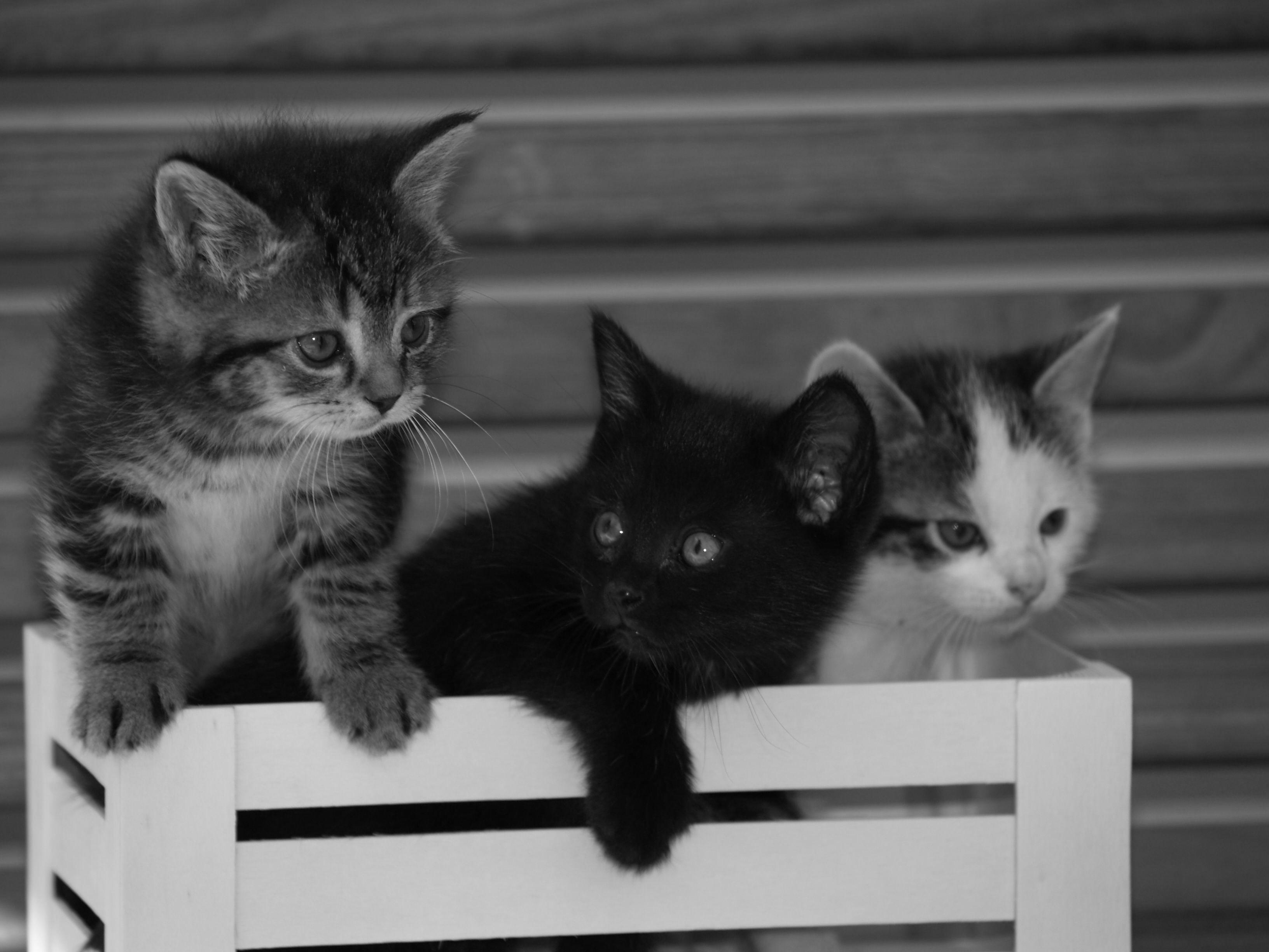
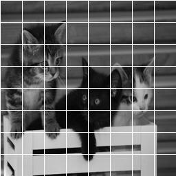
The perceptual hash algorithm, too, initially calculates the gray value image and scales it down. In our case, we desire a factor of 4, which is why we scaled down to 8*4×8*4, that is, a 32×32 image.

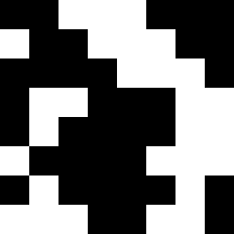
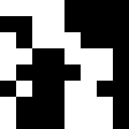
To this image we apply a discrete cosine transform, first per row and afterwards per column.

Discrete cosine transform: 

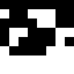
The pixels with high frequencies are now located in the upper left corner, which is why we crop the image to the upper left 8×8 pixels. Next, we calculate the median of the gray values in this image and generate, analogous to the median hash algorithm, a hash value from the image.

Hash: 1010010010101101100110011011001101100010100100000111011010101110

Wavelet Hash

Analogous to the average hash algorithm, the wavelet hash algorithm also generates a gray value image sized 8×8. Next, a two-dimensional wavelet transform is applied to the image. Our tests have revealed that the results improve when we set the top row to 0, that is, to black and re-apply the wavelet transform three times. We took this idea from the image hash library imagehash.

Next, analogous to the perceptual hash algorithm, each pixel is compared to the median and the hash is calculated.

Hash: 0000010110111001111110011111101111111010000000000000011100000101

We took the block hash from the library blockhash-python, implemented the average hash, difference hash, perceptual hash and wavelet hash algorithms based on the imagehash library and developed the median hash algorithm ourselves.

Our Tests

We tested the hash functions against each other using the image database Caltech101 which contains 9143 images. For every image we created 10 individual test images with slight, randomized modifications.

We have:

  • increased and decreased brightness
  • increased and decreased contrast
  • added a watermark
  • converted the image to grayscale
  • scaled it down
  • cropped the borders
  • applied Gaussian smoothing
  • applied JPEG compression

This resulted in 100,584 test images. Next, the individual hashes for each image were calculated and stored along with the image number and the type of error (i. e., the modification applied) in an ElasticSearch index.

We conducted three different tests on each hash:

  1. Grouping by image and counting the number of instances where a hash was calculated that differed from that of the source image.
  2. Grouping by image and calculating the average Hamming distance of a modified image from the source image.
  3. Grouping by hash and counting the number of collisions, that is, the number of images that were assigned the same hash value despite them not belonging to the same source image.

Results

Different hash than the source image

Type of erroraHashbHashdHashmHashpHashwHash
Gaussian smoothing1828 (20.0%)1241 (13.6%)3807 (41.6%)2122 (23.2%)786 (8.6%)971 (10.6%)
Grayscale0 (0%)0 (0%)0 (0%)0 (0%)0 (0%)0 (0%)
Increased brightness3874 (42.4%)3206 (35.1%)5357 (58.6%)3451 (37.7%)3986 (43.6%)2844 (31.1%)
Decreased brightness1717 (18.8%)809 (8.8%)4935 (54.0%)2115 (37.7%)1030 (11.3%)1420 (15.5%)
JPEG compression455 (5.0%)598 (6.5%)1616 (17.7%)658 (7.2%)546 (6.0%)514 (5.6%)
Increased contrast2559 (28.0%)2062 (22.6%)4568 (50.0%)2474 (27.1%)2460 (26.9%)2197 (24.0%)
Decreased contrast2056 (22.5%)766 (8.4%)5223 (51.1%)2154 (23.6%)1063 (11.6%)2026 (22.2%)
Scaled554 (6.1%)1297 (14.2%)2091 (22.9%)851 (9.3%)664 (7.3%)614 (6.7%)
Watermark3600 (39.4%)5046 (55.2%)7167 (78.4%)4029 (44.1%)4242 (46.4%)2896 (31.7%)
Cropped8543 (93.4%)8750 (95.7%)9075 (99.2%)8514 (93.1%)9088 (99.4%)7840 (85.7%)
Total25,186 (25.0%)23,775 (23.6%)43,839 (43.6%)26,368 (26.2%)23,865 (23.7%)21,322 (21.2%)

Average Hamming distance

Type of error

aHash

bHash

dHash

mHash

pHash

wHash

Gaussian smoothing

0.24

0.31

0.61

0.31

0.17

0.20

Grayscale

0.00

0.00

0.00

0.00

0.00

0.00

Increased brightness

0.81

1.22

1.28

0.94

1.14

0.68

Decreased brightness

0.24

0.20

1.15

0.48

0.23

0.31

JPEG compression

0.06

0.13

0.21

0.10

0.12

0.10

Increased contrast

0.38

0.60

0.84

0.43

0.58

0.52

Decreased contrast

0.29

0.59

0.84

0.48

0.23

0.52

Scaled

0.07

0.34

0.28

0.12

0.15

0.12

Watermark

0.64

2.46

2.51

1.30

1.06

0.67

Cropped

4.11

6.02

6.23

4.69

7.47

2.98

Total

0.68

1.14

1.44

0.88

1.12

0.61

Collisions

Hash

Collisions

aHash

4438

bHash

711

dHash

421

mHash

4432

pHash

483

wHash

7866

We also tried to combine the hashes with AND, OR, XOR or with a similarity hash, but the results were at best as good as those of the best of the hashes thus combined.

Calculation duration

Hash

Average calculation duration per image

aHash

2.25 ms

bHash

112.70 ms

dHash

0.33 ms

mHash

0.33 ms

pHash

60.05 ms

wHash

0.91 ms

As the perceptual hash showed good results in overall deviations and the average Hamming distance while producing few false positives and being twice as fast as the block hash algorithm, we opted for the perceptual hash algorithm.